
Original Articles: 2021 Vol: 13 Issue: 2
Application of the Cross-Validation Method to the Calibration Functions in the Validation Process of an Indirect Analysis Method: Determination of Organic Compounds in Water by UV-Visible Spectrophotometry
Chaymae Jermouni, Mohamed Nohair*, Sara Azmi, El Mati Khoumri, Abdelhak Elbrouzi and Mohssine Elmorrakchi
Laboratoire de Chimie Physique and de Chimie Bioorganique, Energie, Electrochimie Interfaciale et Chimiométrie F.S.T de Mohammedia-Maroc Maroc, France
Abstract
In the process of validation of analytical methods, the guides NF T90-210 or NF V03-110 [1,2] are most often used, they are respectively used in chemical analysis of water and the agro-food field. For indirect analysis methods, which is frequently the case and especially for spectroscopic analysis methods, validation takes place after verification of the performance criteria of an appropriate calibration model. The validation or verification of the calibration function in a measurement area depends on the guide used.
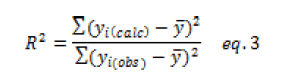
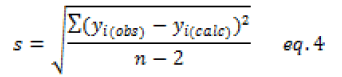
For example, an MAD (Maximum Accepted Deviation) can be proposed for the adjustment between the experimental values and those adjusted by the calibration function. One can also use a statistical test of suitability by a variance study, which compares the residual variance with the variance explained by the proposed model. Statistical indicators such as the coefficient of determination and the standard error (R2; s) of the model are then calculated.
However, these verification methods are insufficient because they do not provide an experimental protocol to test the performance of the proposed model in the prediction phase. It is easy to find a coefficient of determination R2>0.95 for a fit between the observed and calculated values, but it does not guarantee the quality of the results that will be obtained. It is easy to erroneously accept an analytical method as valid in one's field of study because the instrumental response function is not properly defined. As a result, the performance evaluation of the characteristics of the analytical method leads to biased results. In this work, we propose a simple and robust protocol for the verification of the performance of the instrumental response function (calibration model) of an indirect analytical method.
The approach consists in the use of the cross-validation method (80-20%), which is a method commonly used in statistical modeling in chemistry and biology (QSAR and QSPR) [3,4]. Statistical indicators recalculated using this method are more robust and reflect better the suitability of the calibration function and its performance. The analysis method used in this work consisted of measuring the quantity of organic matter using a UV-Visible spectrum between 200 and 300 nm. We used three calibration functions by comparing the statistical indicators, as the coefficient of determination and the residual error (R2, s), which are derived from the cross-validation method of these functions. The fit between the observed and predicted values with respect to an acceptability deviation of 20% was additionally verified.
The obtained results lead to the adoption of a three-wavelength multiple regression model as a fair and robust calibration model. Unfortunately, the limited data available did not allow us to test other more advanced functions as neural networks.
Keywords
Analytical method validation; Calibration function; Cross-validation method; UV visible spectrophotometry; Organic matter
Introduction
The analytical method lifetime is an evolving process that follows different stages [5,6] which can be represented by a cycle illustrated in Figure 1.

Figure 1: The principal phases of the life cycle of an analytical method
Step 1: The analytical method is developed and implemented for its intended purpose. The optimization of all parameters that could influence the measurement process is strongly recommended through the use of experimental designs. Taguchi's approach can also be used to study the robustness of the proposed method [7]. The objective is to reduce the noise effect of all parameters that vary independently of the analyst. This study is very important because it improves the precision of the analytical method. Thus, in this development phase, we can look for the operating conditions for a fair and less dispersive method [8].
Step 2: Validation of the developed method with respect to the expected use using an intra-laboratory characterization as well as an inter-laboratory study if necessary. This study is intended to evaluate the uncertainty of the analytical method.
Step 3: Routine usage of the method may lead to a revalidation requirement. It is sometimes necessary to re-optimize the analytical method due to measurement target deviation or capability degradation. According to EN ISO/CEI 17025 guide [9], the validation of an analytical method is the "confirmation by examination and objective evidence provision that the specific requirements for a given intended use are fulfilled". This confirmation consists of comparing the values of the performance criteria determined during the method characterization study with those expected or assigned beforehand (limits of acceptability, objectives to be achieved) and then declaring the analytical method valid or invalid.
The analytical method characteristics are a set of quality parameters that are assigned to the analytical method and that can be quantified or qualified. These parameters are quantities to be estimated from a set of measurements, e.g. relative bias to indicate accuracy, and repeatability standard deviation to describe the capability of the analytical method. However, the validation criteria for an analytical procedure are a specified limit value established for a performance characteristic. For example, the validation of a method for the quantification of medicinal product residues, according to European regulations, requires a repeatability coefficient of variation ≤ 20% and precision between 70% and 120% with respect the reference value to be measured [10].
In this work, we are focusing on the calibration functions, or instrumental response functions, of indirect analytical methods. They allow the determination of any measurable or non-measurable value of a quantity from an instrumental response by a mathematical model. They have crucial importance since they govern the whole validation process. A misdefined calibration function can cause biased validation characteristics. Analytical methods with weak accuracy can easily be promoted. In the case of indirect analysis methods, it is necessary to express the value of the measured quantity from an instrumental response by using a function f: Y=f(X). Linear functions are the most used model because they are precise and easy to implement using the least-squares method [5]. In the case where deviations from linearity are observed, this disadvantage can be overcome by segmenting the validation domain or by reducing it. Quadratic functions can sometimes be used [11].
In practical terms, there is no requirement imposed on response functions in the analytical method validation process using an indirect analytical method. However, the ability to provide a good fit must be ensured. This is accomplished by using the acceptability limits (Maximum Acceptable Deviations (MAD)) to verify the fit between the observed and model-fitted values. This practice is often used in quality control or forensic metrology and medical biology for blood parameters as well. Furthermore, it is customary to perform a statistical test by a variance study and then calculate the usual statistical indicators such as the coefficient of determination (R2) and the standard root mean square error (s). These methods are not sufficient because they do not allow assessment of the calibration function's performance for measurements that are not part of the learning set. It is therefore easy to incorrectly accept an analytical method as valid in one's field of study because the instrumental response function is not properly defined. In this work, we propose a more rigorous approach using a cross-validation in order to demonstrate the response function's robustness. This consists in decomposing the initial series (the training or learning set) into two subsets, the first one of 80% allows building the calibration model, the second one serves as a test. The process consists in repeating the experiment as many times as necessary to test the totality of the data. Afterwards, we can verify that the deviations between the observed and predicted values are within the acceptable deviation limit (MAD). We also recalculate the usual statistical indicators (R2 and s), coefficient of determination and the root mean square error) of the fit between the observed values and those resulting from the cross-validation method to evaluate the performance of the proposed model.
A comparative study between the verification methods proposed in the two guide’s document cited above and the cross-validation technique (80-20%) is presented for a series of three calibration functions (two simple and multiple linear regression models and a polynomial function). The data are derived from the UV-visible absorption of organic matter in water at three wavelengths (265, 280 and 285 nm).
Experimental and Statistical Study
UV-Visible Spectrophotometry for the Routine Measurement of Organic Compounds in Water
Organic Matter (OM) and nitrate contents are part of regulations defining the good ecological status of a water resource, or its compliance if it is used for drinking water production (Table 1) [12]. However, the determination of organic matter content by conventional analytical methods presents a major handicap linked to the cost of the analyses and the time required to conduct them, in addition to the use of reagents that are environmentally unfriendly. The organic matter content in water is usually measured by determining the CO2 concentration that results from an oxidation reaction of the organic matter present in the water [13]. These impairments inhibit adequate reactivity in pollution cases. It should also be recognized that these standard methods are precise. For this purpose, a focus is being given to the use of other faster methods, such as UV-Visible spectrophotometry [14]. The information offered by this technique is very interesting from a qualitative point of view. It is also interesting from a quantitative perspective, as mathematical methods for data exploration in chemo metrics are developed [15]. For the organic matter content in water, it can be easily determined by UV absorbance or optical density (OD) measurements in the range of 200-300 nm [16].
| Water quality | OM (mg/Litre) |
|---|---|
| Very good | Jusqu’à 20 |
| Good | 25 |
| Average | 40 |
| Poor | 80 |
| Very poor | >80 |
Table 1: Water quality versus organic matter content
As any indirect analysis procedure, a learning set is required to build the calibration model. It consists of several solutions with known organic matter contents in a well-defined range. In this work, six solutions with contents ranging from 10 to 200 mg/L are available [17]. These solutions are prepared from the dissolution of a monopotassium salt of benzene-1, 2-dicarboxylic acid (Phthalic acid, KHP, C8H5KO4) in distilled water (Table 2).
| Solution | 1 | 2 | 3 | 4 | 5 | 6 |
| KHP (mg/L) | 10 | 30 | 50 | 70 | 100 | 200 |
Table 2: Organic matter content of the learning set
The absorbance of the prepared solutions is in the range of 200 to 900 nm. The high absorbance is observed between 200 and 300 nm, which is due to the conjugation present in Phthalic acid [18]. The absorbance at three reliable wavelengths (265, 280 and 285 nm) are used as independent variables, as they show a wider variance depending on the KHP concentrations. A strong correlation was observed between absorbance at the different wavelengths as well as absorbance and organic matter content. The results are reported in Table 3.
| A265 | A280 | A285 | OM | |
|---|---|---|---|---|
| A265 | 1 | |||
| A280 | 0,98 | 1 | ||
| A285 | 0,98 | 0,99 | 1 | |
| MO | 0,96 | 0,91 | 0,95 | 1 |
Table 3: Correlation matrix between absorbance and organic matter content
Results and Discussion
Calibration Models and Statistical Analysis
In the present work, three types of functions were used to implement the calibration models between the organic matter content and absorbance at different wavelengths in UV-Vis. The functions are presented in the following Table 4.
| Function 1 | Simple regression  |
| Function 2 | Quadratic function  |
| Function 3 | Multiple regression  |
Table 4: Proposed calibration models
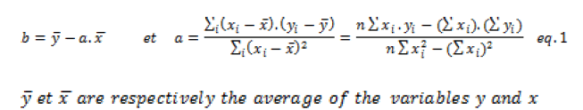
The absorbances at different wavelengths are highly correlated. For the first two models, the absorbance at 265 nm was chosen. The coefficients of the calibration model are estimated using the least-squares method detailed in the literature [5]. For a simple model of the type: Y=a.X+b, total error minimization results in the calculation of the coefficients a and b using the following formulas:
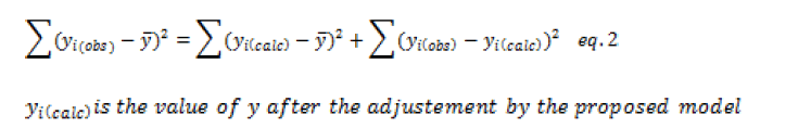
Furthermore, the analysis of variance can be used to decompose the total variation into two components that correspond to the explained variation and the residual variation.
The following table presents the analysis of variance for a simple affine function model (Table 5). (n is the number of measurements and corresponding responses and p=2 is the number of unknowns in the model (a and b)).
| Source | Sum of squares | DDL | Average squares | Ratio |
|---|---|---|---|---|
| Model | 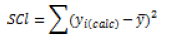 |
2-1 | 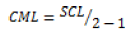 |
 |
| Residual | 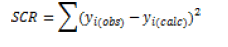 |
n-2 | 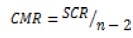 |
|
| Total |  |
n-1 |
Table 5: Analysis of variance for a simple model Y=a.x+b
For a predetermined risk, the Fisher F test compares the ratio F_obs=CML⁄CMR which has been calculated from the previous table with a critical value read on the Fisher-Snedecor table with 1 and (n-2) degrees of liberty. This ratio is always high to select a valid model.
The proportional variation explained by the calibration model in the total variation corresponds to the determination coefficient noted as R2.
As part of a validation of an analytical procedure, the experimental design requires that replicates be performed for reproducibility; the variation decomposition takes another form:
As part of a validation of an ana lytical procedure, the experimental design requires that replicates be performed for reproducibility; the variation decomposition takes another form:
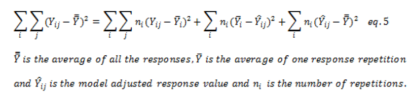
Taking the same decomposition of the total variation to which is added the variation 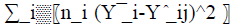 due to the deviation of the model. For a valid model, a Fischer's test must show that the latter is of the same order
as the residual variation. It is important to note that in the majority of cases, this test is very problematic because
the residual variation is very small in spectrophotometric methods of analysis. By using such a test, there is a risk
that the model may be automatically rejected despite its good performance.
due to the deviation of the model. For a valid model, a Fischer's test must show that the latter is of the same order
as the residual variation. It is important to note that in the majority of cases, this test is very problematic because
the residual variation is very small in spectrophotometric methods of analysis. By using such a test, there is a risk
that the model may be automatically rejected despite its good performance.
For verifying the validity of the calibration model through the maximum accepted deviation, a limit value expressed as a percentage is generally proposed in the range of 10-20%.
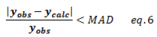
Calibration models are used to recalculate organic content values. The model is valid and accepted when the deviations are less than the limit value. The graph displays in Figure 2 illustrate the accepted calibration model distribution.

Figure 2: Distribution of deviations for a valid calibration model
Analysis and Interpretation
In the first step, a simple model was built using only the absorbance at 265 nm. With respect to statistical indicators, the calibration model is efficient, with a determination coefficient of about 93% (Figure 3). However, the Fischer test shows that the model is very significant. The deviations between calculated and observed values is less than the maximum accepted variance (AMD<20%) (Table 6).
| OMobs | 10 | 30 | 50 | 70 | 100 | 200 |
| OMcalc | 26,22 | 61,07 | 83,08 | 121,60 | 174,4 | |
| Deviation | >> | 12% | 20% | 18% | 21% | 13% |
Table 6: Deviations between calculated and observed values of organic matter content

Figure 3: Adjustment between the observed and calculated values by the linear model
All indications suggest that the model is appropriate and suitable in this case. However, the predictive power of the
model was tested using the cross-validation method (80-20%). The model is constructed from the available data
with a single value being taken as a test. The value of the organic matter content for this data is recalculated from
the model and the operation is repeated as many times to recalculate the organic matter contents for the all data. A
simple model between the observed and calculated values 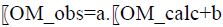 is constructed to re-evaluate
the statistical indicators. The statistical indicators appear less satisfactory with a significantly reduced coefficient
of determination (72%). In addition, deviations between the observed and calculated organic matter values are
very high (Table 7).
is constructed to re-evaluate
the statistical indicators. The statistical indicators appear less satisfactory with a significantly reduced coefficient
of determination (72%). In addition, deviations between the observed and calculated organic matter values are
very high (Table 7).
| OMobs | 10 | 30 | 50 | 70 | 100 | 200 |
| OMcalc | 24,7 | 64,2 | 85,73 | 129,22 | 134,4 | |
| Deviation | >> | 17% | 26% | 22% | 29,2% | 30% |
Table 7: Results of the cross-validation method
The results of the cross-validation indicate the predictive weakness of the proposed model and its lack of widespread use. Therefore, the use of this calibration model may lead to the acceptance of an analytical method with biased accuracy.
In order to improve the fit, a quadratic model is proposed. The least-squares method was used to determine the calibration model coefficients and the same procedure was used to determine the statistical indicators of the model and the deviations between the observed and calculated organic matter content values. Better statistical indicators were found compared to the linear model (Figure 4), with an acceptable fit (Table 8).
| OMobs | 10 | 30 | 50 | 70 | 100 | 200 |
| OMcalc | 22,47 | 48 | 68 | 115 | 193 | |
| Deviation | >> | 20% | 4% | 1,8% | 13,7% | 3,4% |
Table 8: Deviations between the calculated and observed organic matter values for the quadratic model

Figure 4: Adjustment between the observed and calculated values by the quadratic model
Moreover, the results of the cross-validation are still very poor with a decrease in the determination coefficient (91%) and deviations between the calculated and observed values of the organic matter content exceed the maximum accepted deviation of 20% (Table 9). Nevertheless, the results show better results than those of the linear model.
| OMobs | 10 | 30 | 50 | 70 | 100 | 200 |
| OMcalc | 24,7 | 47,2 | 68,73 | 118,22 | 152,40 | |
| Deviation | >> | 24% | 6% | 3% | 20,2% | 23% |
Table 9: Results of the cross-validation method
In the last step, a multiple regression model was considered integrating the absorbance at wavelengths (265,280 and 285 nm). The calibration model coefficients are determined by the least-squares method. As the absorbance values are of the same order of magnitude, there is no need to transform the absorbance values into reduced values. Therefore, these coefficients do not reflect the contribution of each absorbance value since they are highly correlated. However, the model's explanatory component value is of around 99% (R2) and the deviations between the observed and calculated values of the organic matter content are very slight (Table 10).
| OMobs | 10 | 30 | 50 | 70 | 100 | 200 |
| OMcalc | 12,58 | 28,92 | 45,54 | 68,53 | 106,20 | 198,19 |
| Deviation | 25% | 3,5% | 8,9 | 2,1% | 6,2% | 0,009% |
Table 10: Deviations between calculated and observed organic matter values for the multiple regression models
Additionally, the predictive power was tested by cross-validation, and the statistical indicators remain very satisfactory, with a determination coefficient of approximately 94% and deviations of no more than 20% (Table 11). The calibration model using multiple regressions gives better results and is suitable as a calibration model for organic matter determination in water from UV absorbance. Nevertheless, it was noted that the 10 mg/l content is very difficult to integrate into all three models. Instead, it would be more appropriate to use more complex functions or simply reduce the calibration function's use interval. Alternatively, the experiment interval can be split into two or three segments and construct as many calibration models.
| OMobs | 10 | 30 | 50 | 70 | 100 | 200 |
| OMcalc | 18 | 28,09 | 40,91 | 65,73 | 110,22 | 160,39 |
| Deviation | >> | 6,35% | 20% | 0,6% | 10,9% | 19% |
Table 11: Results de the cross-validation method for the multiple regressions
Conclusion
This study has shown that calibration models, which appeared to be valid with respect to the statistical indicators imposed by Fisher's tests and the maximum accepted deviation values defined by certain guides, show a deficiency in their predictive and generalizing power. However, cross-validation (80-20%) allows a better verification of the robustness of the calibration models in the prediction phase, by recalculating the statistical indicators of a simple model between observed values of the organic content in water and those resulting from the cross-validation technique.
Based on three calibration models by measurement of the UV (ultraviolet) absorption at a wavelength of 200 nm ~ 300 nm, the cross-validation method showed the superior performance of a multiple regression model compared to other simple and quadratic regression models with absorbance at a single wavelength (265 nm). The cross-validation method is a powerful technique for the validation and verification of calibration models in the validation process of indirect analytical methods. In this way, this technique allows us to avoid wrongly accepting an analytical method as valid in its field of study as the instrumental response function is not properly defined or has a very poor predictive performance.
References
- NF T90-210 Qualité de l'eau-Protocole d'évaluation initiale des performances d'une méthode dans UN laboratoire, 2018.
- NFV03-110 version-Analyse des produits agricoles et alimentaires-Protocole de caractérisation en vue de la validation d’une méthode d’analyse, 2010.
- M Nohair; D Zakarya; A Berrada. J Chem Inform Computer Sci. 2002, 42(3), 586-591.
- K Roy. Advances in QSAR Modeling: Applications in Pharmaceutical, Chemical, Food, Agricultural and Environmental Sciences. Springer International Publishing AG, 2017
- M Feinberg. Labo-Stat:Guide de validation des méthodes d’analyse, Lavoisier, Tec & Doc, Paris, 2009.
- A Holst-Jensen; KG Berdal. J AOAC Int. 2004, 87(4), 927-36.
- M Pillet. Les Plans d'expériences pour la méthode TAGUCHI, les éditions d’organisations, Paris, 1997
- SLC Ferreira; AO Caires; TDS Borges; AMDS Lima; LOB Silva; LOB Silva. Microchem J. 2017, 131, 163–169.
- NF EN ISO CEI 17025: Exigences particulières concernant la compétence des laboratoires d’étalonnages et d’essais, 2005.
- P Hubert; JJ Nguyen-Huu; B Boulanger. STP Pharma. 2003, 13(3), 101-138.
- S Huet; A Bouvier; MA Poursat ; E Jolivet. Statistical Tools for Nonlinear Regression, Springer Verlag, New-York, 2004.
- World Health Organization. Guidelines for drinking-water quality: recommendations, 1, 1993.
- L Gustavsson; M Engwall. Waste Manag. 2012, 32, 104–109.
- C Baisheng; W Huanan; L Sam Fong. Talanta. 2014, 120, 325-330
- O Thomas; C burgess. UV-visible spectrophotometry of water and wastewater (second edition). Elsevier, 2017.
- C Baisheng; W Huanan; L Sam Fong. Talanta. 2014, 120, 325-330
- C Kim; JB Eom; S Jung; T Ji. Sensors. 2016, 16, 61-67.
- O Thomas; C burgess. UV-visible spectrophotometry of water and wastewater (second edition). Elsevier, 2017